I-JEPA
JEPA is a self-supervised learning method that learns visual representations by predicting representations in abstract latent space, without relying on generative modeling or hand-crafted data augmentations.
Based on paper: I-JEPA: Image-based Joint Embedding Predictive Architecture (Bardes et al., 2023)
See it in action
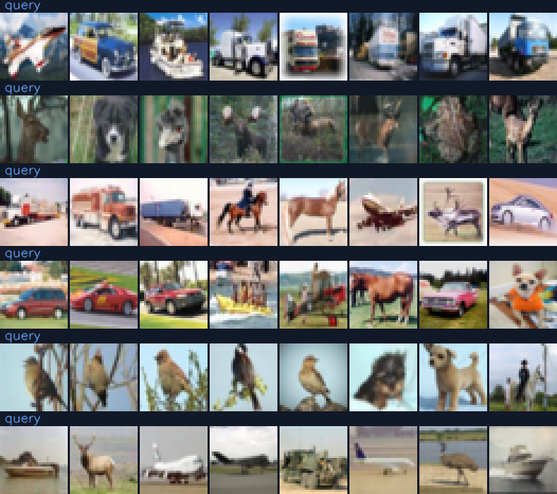
Trained from scratch in one to two hours on a 4 GB laptop GPU with
python demos/jepa_demo.py train, then recorded with python demos/jepa_demo.py record.
More clips are in the gallery.
Overview
I-JEPA learns visual representations without:
- Hand-crafted data augmentations (color jitter, grayscale, etc.)
- Negative examples (contrastive learning)
- Pixel-level reconstruction (autoencoders, MAE)
Instead, it predicts the latent representation of one image region from another region using a Vision Transformer (ViT) backbone. The predictor operates in embedding space, not pixel space, which forces the model to learn semantically meaningful features.
graph TD
    A["Input image x"] --> B["Context encoder f_θ"]
    A --> C["Target encoder f_θ̄ (EMA)"]
    B --> D["Context patches (masked)"]
    C --> E["Target patches"]
    D --> F["Predictor g_φ"]
    E --> G["Target representation sg(y_target)"]
    F --> H["Predicted representation ŷ"]
    H --> I["L2 loss"]
    G --> I
    I --> J["sg: stop-gradient through target encoder"]
Architecture
High-level diagram
JEPA Architecture
Vision Transformer (ViT)
The backbone encoder in simulusion.models.vit is a Vision Transformer
following the standard ViT architecture with JEPA-specific modifications.
Patch embedding:
The input image x ∈ ℝ^{3×H×W} is split into patches of size P × P,
producing N = (H/P) × (W/P) patches. Each patch is linearly projected to
embed_dim:
Transformer blocks:
Each block consists of:
- LayerNorm → Multi-Head Self-Attention → residual
- LayerNorm → MLP (GELU, 4× hidden) → residual
- DropPath (stochastic depth) regularization during training
Key architectural details:
- No class token — all patch tokens are used
- Pre-normalization (LayerNorm before attention and MLP)
- Fixed sin-cos positional embeddings (not learned)
Target Encoder (EMA)
The target encoder f_{\bar{θ}} has the same architecture as the context
encoder f_θ but its weights are an exponential moving average (EMA) of
the context encoder's weights:
where m is the momentum coefficient (default: cosine schedule from 0.996 to
1.0). The target encoder receives stop-gradient.
Predictor
The predictor g_φ is a narrow transformer that predicts target patch
representations from context patch representations. Its width is fixed at 384
channels and its head count is inherited from the backbone; its depth follows
the backbone (Appendix A): 6 layers for ViT-B, 12 for ViT-L/H, 16 for ViT-G.
Leave pred_depth=None to get the paper's depth for the configured backbone.
Key design:
| Property | Detail |
|---|---|
| Lighter than the encoder | Fewer layers, smaller hidden dim |
| Positional embeddings for all patches | The predictor knows which target patches to predict |
| Mask tokens for target positions | Learnable embeddings substituted for masked patches |
Masking
I-JEPA uses multi-block masking: random rectangular blocks are masked rather than individual patches.
config.num_enc_masks = 1  # 1 context block
config.enc_mask_scale = (0.85, 1.0)  # Context covers 85-100% of the image
config.num_pred_masks = 4  # 4 target blocks
config.pred_mask_scale = (0.15, 0.2)  # Each target is 15-20%
config.aspect_ratio = (0.75, 1.5)  # Target block aspect ratio range
The context block is sampled at unit aspect ratio, and every region overlapping a target block is then removed from it, leaving ~25% of the patches visible on average. The predictor sees those context patches and must predict the representation of each target block's patches.
These are not free parameters -- the paper's ablations turn on them:
| Setting | Paper value | Low-shot top-1 if changed |
|---|---|---|
| Target blocks (Table 10) | 4 | 9.0 with 1 block, vs 54.2 |
| Target scale (Table 8) | (0.15, 0.2) | 33.6 at (0.2, 0.3), vs 54.2 |
| Context scale (Table 9) | (0.85, 1.0) | 31.2 at (0.40, 1.0), vs 54.2 |
Training
Loss Function
The I-JEPA loss is the L2 distance between predicted and target representations,
averaged over masked patches (loss_type="l2"; "l2_sum" keeps the paper's
per-block sum, and "smooth_l1" matches the reference implementation):
Optimization
Learning Rate Schedule
Appendix A: linear warmup from start_lr (1e-4) to lr (1e-3) over the first
15 epochs, then cosine decay to final_lr (1e-6). Weight decay is raised
linearly from 0.04 to 0.4 across pretraining, and the EMA momentum from 0.996
to 1.0.
Those learning rates are quoted for the paper's batch size of 2048. Simulusion
scales them linearly by batch_size * world_size / lr_reference_batch_size, so
smaller batches get a proportionally smaller learning rate automatically. Set
lr_reference_batch_size = None to use lr verbatim.
Usage in Simulusion
Quick start
import simulusion

agent = simulusion.create_model(
    "jepa",
    dataset="imagenet",
    batch_size=64,  # the paper uses 2048 across 16 GPUs; the LR follows it
    epochs=100,
)
agent.train()
Using config directly
from simulusion import JEPAAgent, JEPAConfig

cfg = JEPAConfig()
cfg.dataset = "imagenet1k"
cfg.root_path = "/data/imagenet"
cfg.image_folder = "train"
cfg.batch_size = 64
cfg.epochs = 100

agent = JEPAAgent(cfg)
agent.train()
Data pipeline
cfg.dataset = "imagenet1k"  # ImageNet-1K (requires download)
cfg.root_path = "/data/imagenet"

# Or use a generic image folder:
cfg.dataset = "imagefolder"
cfg.root_path = "./my_dataset"
cfg.image_folder = "train"

# Or CIFAR-10 for testing:
cfg.dataset = "cifar10"
cfg.download = True
Note
I-JEPA uses no hand-crafted view augmentations -- that is the paper's
central claim. use_horizontal_flip, use_color_distortion and
use_gaussian_blur all default to False, leaving only the random resized crop
of the reference implementation. Turning them on departs from the paper.
CLI
simulusion train jepa --dataset imagenet1k --epochs 100 --batch_size 64See Configs for the full JEPAConfig field reference with defaults.
Inference and Downstream Tasks
I-JEPA is evaluated with a frozen encoder. Load the EMA target-encoder -- the one the paper evaluates -- and average-pool its patch tokens:
import torch
from simulusion.training.eval_jepa import load_jepa_encoder

device = torch.device("cuda" if torch.cuda.is_available() else "cpu")
encoder = load_jepa_encoder("results/jepa/jepa_run-latest.pth.tar", device)

with torch.no_grad():
    representations = encoder(images).mean(dim=1)  # [batch, embed_dim]
Linear probing protocol
simulusion.training.eval_jepa implements Appendix A.2: the encoder is
frozen, features are the average-pooled patch tokens (I-JEPA has no [cls]
token), and a linear head is trained on them with LARS for 50 epochs at batch
16384, decaying the learning rate 10x every 15 epochs. It sweeps reference
learning rates [0.01, 0.05, 0.001], weight decays [0.0005, 0.0], the
average-pooled last layer against the concatenated last four layers, and a head
with and without a preceding batch-norm, reporting the best.
simulusion eval --model jepa \
    --checkpoint results/jepa/jepa_run-latest.pth.tar \
    --root-path /data/imagenet --model-name vit_base --output probe.json

# equivalent, without the CLI wrapper
python -m simulusion.training.eval_jepa \
    --checkpoint results/jepa/jepa_run-latest.pth.tar \
--root-path /data/imagenet --model-name vit_basefrom simulusion.training.eval_jepa import jepa_linear_probe
results = jepa_linear_probe(
checkpoint="results/jepa/jepa_run-latest.pth.tar",
root_path="/data/imagenet",
)
print(results["top1"], results["sweep"])Paper reference points on ImageNet-1K linear evaluation (Table 1):
| Method | Arch. | Epochs | Top-1 |
|---|---|---|---|
| I-JEPA | ViT-B/16 | 600 | 72.9% |
| I-JEPA | ViT-L/16 | 600 | 77.5% |
| I-JEPA | ViT-H/14 | 300 | 79.3% |
| MAE | ViT-B/16 | 1600 | 68.0% |
| data2vec | ViT-L/16 | 1600 | 77.3% |
I-JEPA vs V-JEPA
| Aspect | I-JEPA (Image) | V-JEPA (Video) |
|---|---|---|
| Input | Single image | Video clip |
| Masking | Spatial block masking | Spatio-temporal tube masking |
| Task | Predict masked patch latents | Predict future frame latents |
| Predictor | Transformer | Spatio-temporal transformer |
Common Pitfalls
Predictor collapse
The predictor outputs a constant regardless of input.
Fixes:
- Ensure EMA starts close to 1.0 (default: 0.996)
- Verify predictor output variance is non-zero
Representation collapse
All patches map to nearly identical representations.
Fixes:
- Use multi-block masking (not random patch masking)
- Check the feature covariance matrix
Memory usage
ViT-B/16 with 224×224 creates 196 patch tokens. Batch size 64 requires ~16 GB GPU.
Tips:
- Enable
gradient_checkpointing = True - Reduce
batch_sizeand increaseaccum_iter
Slow convergence
JEPA requires long warmup (40 epochs) and many total epochs (100–300).
Tips:
- Use the cosine schedule for EMA momentum
- Expect 48+ hours on 4× GPUs for ViT-B/16 at 100 epochs
Comparison to Other Methods
| Method | What it predicts | Approach |
|---|---|---|
| Autoencoder | Pixels | Reconstruction |
| VAE | Pixels | Generative |
| MAE | Pixels | Masked modeling |
| JEPA | Latents | Predictive coding |
| IRIS | Tokens | Transformer dynamics |
See Also
- IRIS — discrete world model using JEPA-style token prediction
- Vision Components — ViT encoder and video tokenizer components
References
- Bardes, A., Ponce, J., & LeCun, Y. (2023). I-JEPA: Image-based Joint Embedding Predictive Architecture. arXiv:2301.08243.
- Assran, M., et al. (2023). Self-Supervised Learning from Images with a Joint-Embedding Predictive Architecture. CVPR 2023.
- Dosovitskiy, A., et al. (2021). An Image is Worth 16x16 Words: Transformers for Image Recognition at Scale. ICLR 2021.
Updated Oct 11, 2026